Forecasting Tomorrow’s Demand in the SADI: 2.5 % Error, and Where It Fails

A day-ahead forecast of Argentine hourly demand with gradient boosting, tested on a year the model never saw: how it compares with simple references, what each group of variables contributes, how honest its uncertainty bands are, and which days it gets wrong.

Second study of the series “Reading the SADI with data”. The first one measured how demand responds to temperature.

NoteResumen en castellano

¿Qué tan bien se puede pronosticar la demanda horaria de mañana del SADI con datos públicos? Un modelo de gradient boosting, probado sobre un año que nunca vio (julio 2025 – julio 2026):

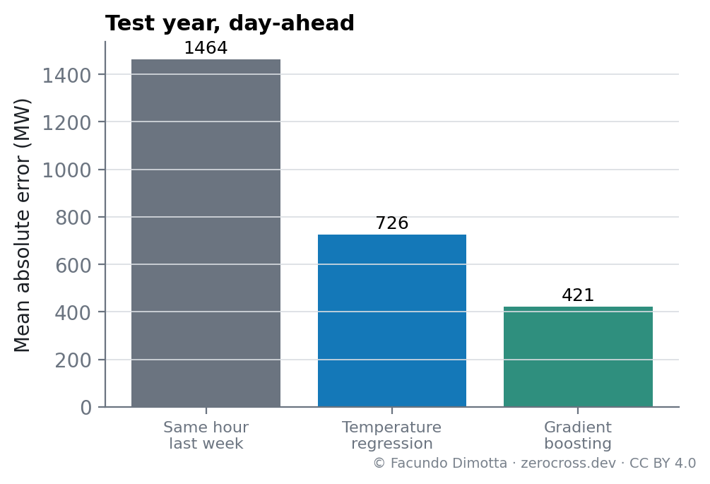
• Error medio de 421 MW (2,5 %), contra 1.464 MW de copiar la semana anterior y 726 MW de una regresión con la temperatura.
• Sin variables meteorológicas, el error se más que duplica. Se usó el clima real, como si el pronóstico del tiempo fuera perfecto: es un límite superior de calidad.
• El punto débil son las fiestas de fin de año (unos 920 MW de error). En el Mundial 2026, la demanda cayó 1 a 2 GW durante los partidos de Argentina.
• Las bandas de incertidumbre calibradas contienen el valor real el 81,7 % del tiempo (objetivo: 80 %).

The question

How well can tomorrow’s hourly demand of the Argentine interconnected system be forecast with public data and a standard machine-learning model? And, just as important: compared with what, and where does it fail?

A forecast is only useful if its error is measured honestly: on data the model has never seen, against simple references, and day by day, so that its weak spots are visible.

Setup

What is forecast. At 10:00 of day D−1, the 24 hourly values of total demand of day D (the sum of the 22 provinces of the SADI).

What the model knows at that moment:

• demand up to day D−2 (day D−1 is still in progress);
• the calendar of day D (working or non-working day, holidays and the days around them);
• the weather of day D.

An important simplification: the weather used is the actual weather of day D (ERA5 reanalysis), as if the weather forecast were perfect. The results therefore measure the error of the model itself; a real forecast adds the error of the weather forecast (see the discussion).

Data split. The model is trained on 2021–2024. The first half of 2025 is used only to choose the model settings and to calibrate the uncertainty bands. The test period, July 2025 to July 2026 (9,504 hours), is used for nothing else: the model never saw it.

Model. Gradient boosting (scikit-learn’s HistGradientBoostingRegressor) on calendar, weather and recent-demand variables. Trees cannot extrapolate a level they have not seen, and demand grows year after year, so the model is set up to follow that growth.

References. A model is only as good as what it beats:

• same hour last week, the simplest possible forecast;
• temperature regression: the piecewise model of the previous study, fitted hour by hour.

Results

Against the references

Day-ahead errors over the test year (July 2025 – July 2026).

Model	Mean absolute error	MAPE	Error in the daily peak
Same hour last week	1,464 MW	8.9 %	1,722 MW
Temperature regression	726 MW	4.5 %	780 MW
Gradient boosting	421 MW	2.5 %	531 MW

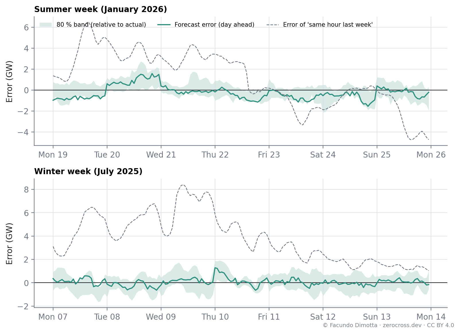
The model cuts the error of the temperature regression by 42 % and that of the weekly persistence by 71 % (Figure 2). Without weather information, its error more than doubles: temperature is the core of the forecast, as the previous study anticipated. Its bias is −183 MW: on average it slightly under-forecasts, consistent with demand growing faster during the test year than in the training years.

Figure 1: Forecast error (forecast minus actual) over two weeks of the test year, with the 80 % band expressed relative to the actual value (the actual demand is inside the band when the band crosses zero), and the error of the weekly-persistence reference. In the winter week, the previous week was a cold wave, and simply copying it misses by several GW.

Figure 2: Mean absolute error of each model over the test year.

Where it fails

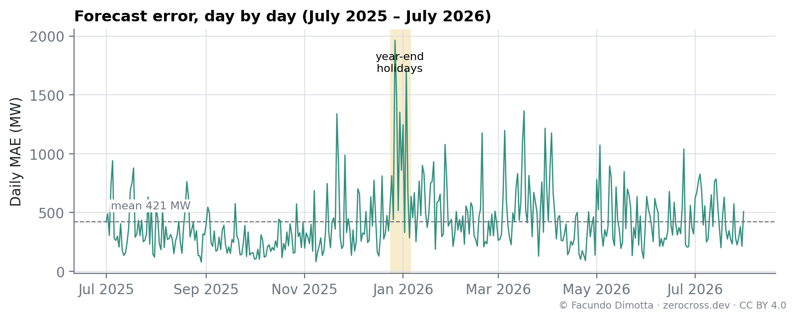
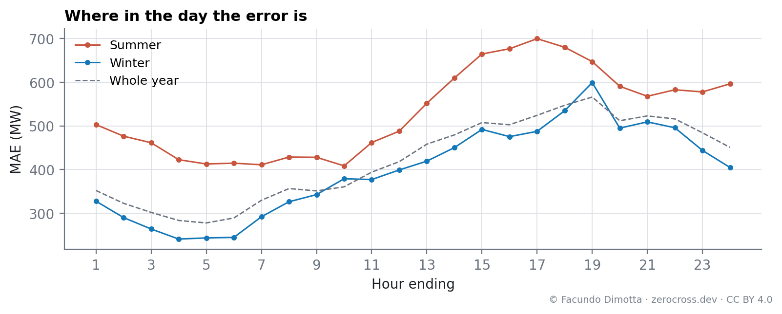
The error is not uniform (Figure 3, Figure 4):

• By season: 532 MW in summer and 468 MW in autumn, against 397 MW in winter and 297 MW in spring. Summer afternoons are the hardest hours, at about 700 MW.
• By day type: 409 MW on working days and 447 MW on non-working days.
• The year-end holidays are the weak spot. Four of the five worst days of the test year fall between 27 December and 3 January, with errors close to 2,000 MW; over the whole holiday period the error averages about 920 MW. The training data contain only four year-end periods, each different, too few for the model to learn them.
• The winter of 2026 brought the largest misses outside the holidays: on 24 June and on 13–14 July demand exceeded the forecast by up to 2 GW. Those were polar-air days with clear, calm nights, and the weather stations of the Servicio Meteorológico Nacional show where the cold was. On 13 July the minimum fell below zero in the suburbs of Greater Buenos Aires (−2.5 °C at El Palomar, −1.7 °C at La Plata, −0.8 °C at Ezeiza) while the City stayed at 3–4 °C, and the daily mean of the suburban stations was 2–3 °C below the City’s. The model’s only weather point for the province of Buenos Aires is the City, where the urban heat island is strongest on exactly these nights: it did not “see” the cold where most of the demand is. The national daily mean itself was not extreme (about 9 °C in both the reanalysis and the stations).
• The 2026 World Cup (11 June to 19 July) left a clear signature on the days Argentina played: a window of two to three hours in which demand fell 1–2 GW below the forecast, while the rest of the day behaved as usual. The largest drop, 2.2 GW, came during the final on 19 July. The width of the windows matches the length of a match, consistent with commercial and industrial activity pausing while people watch. The model knows nothing about matches, and confirming the attribution hour by hour requires the kick-off times.
• The under-forecast bias was about −250 MW before, during and after the tournament alike. It reflects a jump in the weather-corrected level of demand in 2026 (about +3 % over 2025, faster than in the training years), not the World Cup. Correcting the forecast with its own recent errors, which are known at issue time, is the standard remedy and the next improvement to test.

Figure 3: Mean absolute error of each day of the test year. Shaded: the year-end holidays.

Figure 4: Mean absolute error by hour of the day, for summer, winter and the whole year.

How honest the uncertainty is

Along with the central forecast, the model gives a band that should contain the actual value 80 % of the time. The first version of the band, built directly from quantile models, contained it only 52 % of the time: the model was more confident than it should be. After a standard calibration with the first half of 2025 (conformalized quantile regression), which widens the band by about 300 MW, it contains the actual value 81.7 % of the time over the test year, with an average width of about 1,400 MW.

Discussion

• Day-ahead demand is predictable to within about 2.5 % with public data and a standard model, provided the weather forecast is good. Most of the difficulty is in the weather.
• This is an upper bound on quality, not a real-world figure. With more than 1,000 MW per degree on summer afternoons (previous study), a temperature forecast that misses by one or two degrees adds an error comparable to the whole error of the model. The next step is to repeat the test with archived weather forecasts instead of actual weather.
• A comparison with the system operator’s official day-ahead forecast is the natural benchmark, but its historical forecasts are not in the databases used here.
• Knowing when not to trust the model is part of the result: around the year-end holidays its error is more than twice the usual, and a user of the forecast should know it.

Limitations

• Perfect weather, as explained above.
• National total only; the provincial forecast, and the split between distributors and large users, are not evaluated here.
• The target is the demand of the provinces, which excludes transmission losses (about 3–4 %; they are reported monthly, and hourly only until 2022). Forecasting the generation needed would require adding them, for example with a separate model, since losses grow roughly with the square of the load.
• Exceptional events (major football matches, strikes, very large outages) are not modeled. Nor is the spread of temperature within a province: on cold, calm nights the suburbs of Greater Buenos Aires can be 2–3 °C colder than the City, the model’s only weather point for that province.
• One test year. A different year, with a different summer or a different economic context, would give somewhat different numbers.

Data: this study analyses electricity market data and shows only the results of that analysis (estimates, error measures, statistics, indices and conclusions), not the underlying data; sources and terms of use on the legal page. Weather: Open-Meteo.com and ERA5, Copernicus Climate Change Service (CC BY 4.0); station data of the Servicio Meteorológico Nacional (CC BY 2.5 Argentina) for the winter of 2026.